In the past 100 years, scientists have imagined new ways of boosting the capacity of wireless channels. Around the middle of 20th century, we began to truly understand the role of fundamental players in this equation, namely power and bandwidth. It was realized that the capacity of a wireless channel increases logarithmically with SNR and hence quickly approaches the region of diminishing returns. Nevertheless, with a few exceptions, almost all the research was exclusively focused on single antenna systems. It was only in mid 1990s that the power of using multiple antennas at both ends of the link was discovered. It turned out that the capacity increases linearly with the number of antennas (minimum of Tx and Rx antennas to be exact), even on a single device! This came as a remarkable result at that time but the dots now connect (as always) so easily in the backward direction.
Along with OFDM, multiple antennas have been the driving force behind increasing data rates in spatial multiplexing mode. For this purpose, independent data streams are sent through different antennas in parallel. Since the signals overlap each other, the question is how these independent streams are detected at the Rx side. We explore the answer in this article.
Spatial Multiplexing
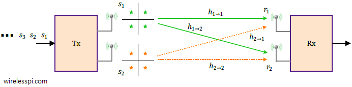
A block diagram for a multiple antenna system with $N_T$ Tx antennas and $N_R$ Rx antennas is drawn in the figure below. In this spatial multiplexing mode, separate bits modulated as $s_1$, $s_2$, $\cdots$, $s_{N_T}$, are simultaneously sent through their respective Tx antennas. For example, for $N_T=2$, the first antenna sends $s_1$, $s_3$, $s_5$, $\cdots$ while the second antenna transmits $s_2$, $s_4$, $s_6$, $\cdots$.

The channel gain between $i$-th Tx antenna and $j$-th Rx antenna is denoted by $h_{(i\rightarrow j)}$. Observe on the Rx side of the above figure that the cumulative signal at each antenna is a summation of signals arriving from all Tx antennas.
$$\begin{equation}
\begin{aligned}
r_j = h_{(1\rightarrow j)}\cdot s_1 + h_{(2\rightarrow j)}\cdot s_2 + \cdots + h_{(N_T\rightarrow j)}\cdot s_{N_T} + \text{noise}, \qquad \\
\qquad j = 1, 2, \cdots,N_R
\end{aligned}
\end{equation}\label{equation-sp-general}$$
These equations can be written into a matrix form as
\begin{equation}\label{equation-r-matrix}
\mathbf{r=H\cdot s+\text{noise}}
\end{equation}
where
- $\mathbf{r}$ is a vector consisting of elements $r_j$, i.e., the signals arriving at Rx antennas
- $\mathbf{s}$ is a vector consisting of the modulation symbols $s_i$
- $\mathbf{H}$ is a matrix of channel coefficients
Since the signals from all Tx antennas arrive at each Rx antenna, the main task of the detection algorithms here is to free each modulated bit sent by one Tx antenna from the interference of the other modulated bits sent by rest of the Tx antennas. Today, we describe the most commonly used linear algorithm, known as Zero-Forcing (ZF), to accomplish this task.
Channel State Information (CSI)
In a tutorial on Singular Value Decomposition (SVD), we saw MIMO detection algorithms for the situation where the channel knowledge is available at the Tx. In such a scenario, a MIMO system in spatial multiplexing mode can be visualized as a transformation of the channel cloud into virtual parallel channels, similar to the independent pipes in the air shown in that tutorial. With channel information absent at the Tx, we talk about the open-loop mode, in which no feedback is received from the Rx indicating the channel conditions.
Zero-Forcing Detector
Linear detectors, as the name says, perform linear operations on incoming signals $r_j$ in Eq (\ref{equation-sp-general}). Since computationally complex algorithms lead to faster battery drainage, linear detectors are attractive due to their simplicity in terms of algorithmic computations. There are two main kinds of linear detectors:
- Zero-Forcing (ZF), and
- Minimum Mean Square Error (MMSE)
Here, we will mainly focus on the Zero-Forcing detector, not only because it is the simpler of the two but also MMSE detection demands a background knowledge of probability theory which is outside the scope of this article. Nevertheless, we will touch upon the modification required to transform a Zero-Forcing solution into an MMSE one.
General Solution
For a system with a single antenna both at the Tx and the Rx, we can write the received signal as
\begin{equation}\label{equation-single-flat-channel-sm}
r = h\cdot s + \text{noise}
\end{equation}
where $s$ is the modulation symbol sent and $h$ is the flat fading channel gain. Multiple observations can be joined together into a matrix. Compare the above expression with Eq (\ref{equation-r-matrix}); they are quite similar! Since the matrix expression could look complicated, we explain the separation procedure of two spatial streams using Zero-Forcing solution. To start, refer to the example from a grade 6 algebra lesson below.
Example from Grade 6 Algebra
You can understand the working of the Zero-Forcing algorithm easily if you can solve the following set of equations for two numbers $s_1$ and $s_2$.
\begin{align*}
2\cdot s_1 + 7\cdot s_2 &= -1 \\
4\cdot s_1 – 5\cdot s_2 &= 17
\end{align*}
Multiply the first equation with $2$ and subtract the second equation.
\[
19\cdot s_2 = -19
\]
The result is $s_2=-1$ and $s_1=3$. This example will now help you in decoding of two spatial streams next, as this can be applied to the individual detection of modulation symbols in spatial multiplexing mode.
Two Layers
As a first step, the figure below illustrates the block diagram of a MIMO system with $N_T=2$ and $N_R=2$ antennas. Both Tx antennas send separate modulation symbols $s_1$ and $s_2$, respectively. From Eq (\ref{equation-sp-general}), we can write the expressions for the two signals at the Rx antennas as
$$\begin{equation}
\begin{aligned}
r_1 &= h_{(1\rightarrow 1)}\cdot s_1 + h_{(2\rightarrow 1)}\cdot s_2 + \text{noise} \\
r_2 &= h_{(1\rightarrow 2)}\cdot s_1 + h_{(2\rightarrow 2)}\cdot s_2 + \text{noise}
\end{aligned}
\end{equation}\label{equation-sp-2×2}$$

This system of equations can be solved like any two equations in algebra. Multiplying the first equation above with $h_{(2\rightarrow 2)}$ and the second equation with $h_{(2\rightarrow 1)}$, we get
\begin{equation*}
\begin{aligned}
h_{(2\rightarrow 2)}\cdot r_1 &= h_{(2\rightarrow 2)} \cdot h_{(1\rightarrow 1)}\cdot s_1 + \require{cancel}\cancel{h_{(2\rightarrow 2)}\cdot h_{(2\rightarrow 1)}\cdot s_2} + \text{noise} \\
h_{(2\rightarrow 1)}\cdot r_2 &= h_{(2\rightarrow 1)}\cdot h_{(1\rightarrow 2)}\cdot s_1 + \require{cancel}\cancel{h_{(2\rightarrow 1)}\cdot h_{(2\rightarrow 2)}\cdot s_2} + \text{noise}
\end{aligned}
\end{equation*}
where the cross-terms are canceled through subtraction. We can thus write
\[
h_{(2\rightarrow 2)}\cdot r_1 – h_{(2\rightarrow 1)}\cdot r_2 = \Big\{h_{(2\rightarrow 2)}\cdot h_{(1\rightarrow 1)} – h_{(2\rightarrow 1)}\cdot h_{(1\rightarrow 2)}\Big\}\cdot s_1 + \text{noise}
\]
which yields the estimate of $s_1$ — denoted as $\hat s_1$ — as
\begin{equation}\label{equation-zf-s1}
\hat s_1 = \frac{h_{(2\rightarrow 2)}\cdot r_1 – h_{(2\rightarrow 1)}\cdot r_2}{h_{(2\rightarrow 2)}\cdot h_{(1\rightarrow 1)} – h_{(2\rightarrow 1)}\cdot h_{(1\rightarrow 2)}}
\end{equation}
For known normalized channel gains and a zero noise scenario, this estimate $\hat s_1$ maps exactly on one of the modulation symbols. When noise or other distortions are present, a 16-QAM example is also shown below where the blue point $\hat s$ gets pulled to the nearest star for a decision. This is due to Gaussian nature of noise distribution.

To find $\hat s_2$ (the estimate of $s_2$), multiply the first equation in Eq (\ref{equation-sp-2×2}) with $h_{(1\rightarrow 2)}$ and the second equation with $h_{(1\rightarrow 1)}$. After subtracting the first equation from the second, $\hat s_2$ is given as
\[
\hat s_2 = \frac{-h_{(1\rightarrow 2)}\cdot r_1 + h_{(1\rightarrow 1)}\cdot r_2}{h_{(2\rightarrow 2)}\cdot h_{(1\rightarrow 1)} – h_{(2\rightarrow 1)}\cdot h_{(1\rightarrow 2)}}
\]
Since both $\hat s_1$ and $\hat s_2$ are found through elimination of the other symbol, we conclude that a Zero-Forcing detector fully eliminates spatial interference from the Tx signal. The result can be generalized to any number of Tx and Rx antennas in a MIMO system where the number of Tx antennas $N_T$ does not necessarily have to be equal to the number of Rx antennas $N_R$.
In a similar manner, a matrix equation for the received signal in the presence of multiple antennas can be written as
\[
\mathbf{r} = \mathbf{H}\cdot \mathbf{s} + \textbf{noise}
\]
where $\mathbf{r}$ is the received signal vector at all $N_R$ antennas, $\mathbf{H}$ is the channel matrix composed of coefficients $h_{(i\rightarrow j)}$ while $\mathbf{s}$ is the vector of modulation symbols. Generalizing the two layers solution above, the Zero-Forcing solution was derived here as
\begin{equation}\label{equation-zf}
\mathbf{\hat s} = \mathbf{\left(H^*H\right)^{-1}}\mathbf{H^{*}}\cdot\mathbf{r}
\end{equation}
Some relevant comments are in order now.
Channel Estimation: The channel estimates $h_{(1\rightarrow 1)}$, $h_{(1\rightarrow 2)}$, $h_{(2\rightarrow 1)}$ and $h_{(2\rightarrow 2)}$ are initially not known at the Rx which in practice need to be obtained through a known training sequence or pilot symbols embedded in the sent message. In most infrastructure based systems like 5G and WiFi at microwave frequencies, this has become a relatively easy problem to solve.
Diversity Order: Recall that diversity order refers to the negative slope of the BER curve on a logarithmic plot. Consequently, the higher the diversity order, the lower the BER curve. In Zero-Forcing algorithm, from the viewpoint of one stream (e.g., for $s_1$ above), the energy from the other modulation symbols (e.g., from $s_2$ above) is treated as an interference nulling problem. This null forcing implies that the diversity order of the Zero-Forcing solution is $1$ in the current scenario. For a general MIMO system with $N_T$ Tx antennas and $N_R$ Rx antennas where $N_R>N_T$, the Zero-Forcing algorithm has a diversity order of $N_R-N_T+1$. This is because $N_T-1$ dimensions at the Rx are employed for removal of spatial interference while the rest $N_R-N_T+1$ provide the diversity gain.
Noise Enhancement: Notice that we ignored the role of noise in the above calculations. Looking back at Eq (\ref{equation-zf-s1}), the denominator $h_{(2\rightarrow 2)}\cdot h_{(1\rightarrow 1)}$ $-$ $h_{(2\rightarrow 1)}\cdot h_{(1\rightarrow 2)}$ appears with the noise terms too. For example, from Eq (\ref{equation-single-flat-channel-sm}),
\[
\begin{aligned}
\frac{h^*}{|h|^2}\cdot r &= \frac{h^*}{|h|^2}h\cdot s + \frac{h^*}{|h|^2}\text{noise} \\ &= s + \frac{h^*}{|h|^2}\text{noise}
\end{aligned}
\]
Consequently, the channel gains with low values in this denominator $|h|^2$ severely amplify the noise, a phenomenon known as noise enhancement creating bad spatial sub-channels. Results in trial experiments have shown poor performance by the Zero-Forcing solution, particularly in previous generations of cellular networks where there is abundant interference present from other users. This, however, changes with a very large number of antennas at the base station or massive MIMO systems, the driving technology behind 5G standard. In that setup, Zero-Forcing is the dominant technique for interference cancellation.
Minimum Mean Square Error (MMSE) Detector
Due to the noise enhancement problem, a Minimum Mean Squared Error (MMSE) solution is often preferred in which noise variance is also taken into account before the matrix inversion. Compared with the Zero-Forcing solution in Eq (\ref{equation-zf}), an MMSE solution is given by
\begin{equation*}
\mathbf{\hat s} = \mathbf{\left(H^*H+\sigma^2\mathbf{I}\right)^{-1}}\mathbf{H^{*}}\cdot\mathbf{r}
\end{equation*}
where $\sigma^2$ represents noise power and $\mathbf{I}$ is an identity matrix. Non-zero noise power prevents very low values in the inversion process. This is a compromise between noise enhancement and spatial interference suppression.
Finally, there are better performing non-linear algorithms that outperform linear algorithms at a cost of computational complexity such as Successive Interference Cancelation (SIC) and maximum likelihood detection.
if its full paper with code function better
Hi Qasim,
Thanks for the article.
All makes sense until final estimate equations for s1 or s2… How do get all those (h) values?
Thanks
Kadhiem
The channel gains are assumed known in MIMO detection algorithms which is accomplished by a preceding training phase where known symbols are sent to the Rx to assist in estimation procedure.