We learned in the concept of frequency that most signals of practical interest can be considered as a sum of complex sinusoids oscillating at different frequencies. The amplitudes and phases of these sinusoids shape the frequency contents of that signal and are drawn through magnitude response and phase response, respectively. In DSP, a regular goal is to modify these frequency contents of an input signal to obtain a desired representation at the output. This operation is called filtering and it is the most fundamental function in the whole field of DSP.
It is possible to design a system, or filter, such that some desired frequency contents of the signal can be passed through by specifying $H(k) \approx 1$ for those values of $k$, while other frequency contents can be suppressed by specifying $H(k) \approx 0$. The terms lowpass, highpass and bandpass then make intuitive sense that low, high and band refer to desired spectral contents that need to be passed while blocking the rest.
Filter Frequency Response
The figure below shows the magnitude response $|H(F)|$ (as a function of continuous frequency) of an ideal lowpass filter. A lowpass filter passes frequencies near $0$ while blocks the remaining frequencies.
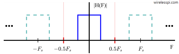
As explained in the discussion about sampling, in a continuous frequency world, the middle filter is all that exists. However, in a sampled world, the frequency response of the filter — just like a sampled signal — repeats at intervals of $F_S$ (sampling frequency) and there are infinite spectral replicas on both sides shown with dashed lines. The primary zone of the sampled frequency response is from $-0.5F_S$ to $+0.5F_S$ shown within dotted red lines with its spectral contents in solid line. From the article on sampling, we know that filter response near $0$ is the same as that near $F_S$ and the filter response around $+0.5F_S$ is the same as around $-0.5F_S$.
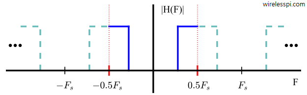
On the other hand, a highpass filter passes both positive and negative frequencies near $0.5F_S$ while blocking everything else. Observe the symmetry around $\pm 0.5F_S$ in Figure below. Similarly, bandpass filters only pass a specific portion of the spectrum.
Filter Impulse Response
Since a filter is a system that modifies the spectral contents of a signal, it naturally has an impulse response $h[n]$ just like a system. When this impulse response is finite, the filter is called Finite Impulse Response (FIR). Impulse response $h[n]$ of an FIR filter, i.e., the sequence of its coefficients, can be found by taking the iDFT of the frequency response $H[k]$.
FIR Filter Design
Understanding of FIR filter design starts from the following argument for continuous frequency domain. Since ideal filters have unity passband and zero stopband and a direct transition between these two, this finite frequency domain support produces an impulse response $h[n]$ in time domain which is infinite and hence non-realizable, as explained in the discussion about frequency. When this $h[n]$ is truncated on the two sides, it is equivalent to multiplication of the ideal infinite $h[n]$ by a rectangular window $w_{\text{Rect}}[n]$ as
\begin{equation*}
h_{\text{Truncated}}[n] = h[n] \cdot w_{\text{Rect}}[n]
\end{equation*}
As mentioned previously, windowing is a process of pruning an infinite sequence to a finite sequence. We know that multiplication in time domain is convolution in frequency domain, and that the spectrum of a rectangular window is a sinc signal. Thus, convolution between the spectrum of the ideal filter and this sinc signal generates the actual frequency response $H(F)$ of the filter.
\begin{equation*}
H(F) = \text{Ideal brickwall response} * sinc(F)
\end{equation*}
This sinc signal has decaying oscillations that extend from $-\infty$ to $\infty$. Convolution with these decaying oscillations is the reason why a realizable FIR filter always exhibits ripple in the passband and in the stopband as well as a transition bandwidth between the two. Naturally, this transition bandwidth is equal to the width of the sinc mainlobe, which in turn is a function of the length of the rectangular window in time. Truncation with a rectangular window causes the FIR filters to have an impulse response $h[n]$ of finite duration.
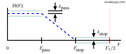
Sidelobes appearing in the stopband of the filter, transition bandwidth and ripple in the passband characterize the performance of a filter. These parameters are usually specified in terms of decibels (or dBs). The filter magnitude in dB is given by
\begin{equation*}
|H(F)|_{dB} = 20 \log_{10} |H(F)|
\end{equation*}
It should be remembered that the multiplicative factor $20$ above is replaced by $10$ for power conversions (because power is a function of voltage or current squared). The advantage of converting magnitudes to dBs for plotting purpose is that very small and very large quantities can be displayed clearly on a single plot.
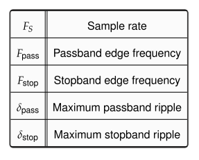
A filter is designed in accordance with the parameters in Table below and shown graphically in the next Figure.
FIR filter design basically requires finding the values of filter taps (or coefficients) that translate into a desired frequency response. Many software routines are available to accomplish this task. A standard method for FIR filter design is the Parks-McClellan algorithm. The Parks-McClellan algorithm is an iterative algorithm for finding the optimal FIR filter such that the maximum error between the desired frequency response and the actual frequency response is minimized. Filters designed this way exhibit an equiripple behavior in their frequency responses and are sometimes called equiripple filters (equiripple implies equal ripple within the passband and within the stopband, but not necessarily equal in both bands).
We design a lowpass FIR filter through Parks-McClellan algorithm in Matlab that meets the following specifications.
\begin{align*}
&\text{Sample rate}, \quad F_S = 12\: \text{kHz} \\
&\text{Passband edge} \quad F_{\text{pass}} = 2\: \text{kHz} \\
&\text{Stopband edge} \quad F_{\text{stop}} = 3\: \text{kHz} \\
&\text{Passband ripple} \quad \delta_{\text{pass,dB}} = 0.1\: \text{dB} \\
&\text{Stopband ripple} \quad \delta_{\text{stop,dB}} = -60\: \text{dB}
\end{align*}
First, noting from above Figure that the maximum amplitude in the passband of frequency domain is $1+\delta_{\text{pass}}$, we can convert dB units into linear terms as
\begin{align*}
20 \log_{10} \big(1+\delta_{\text{pass}}\big) &= \delta_{\text{pass,dB}} \\
1+\delta_{\text{pass}} &= 10^{\delta_{\text{pass,dB}}/20} \\
\delta_{\text{pass}} &= 0.012
\end{align*}
For the stopband,
\begin{align*}
20 \log_{10} \delta_{\text{stop}} &= \delta_{\text{stop,dB}} \\
\delta_{\text{stop}} &= 10^{-60/20} = 0.001
\end{align*}
A Matlab function firpm() returns the coefficients of a length $N+1$ linear phase (which implies real and symmetric coefficients) FIR filter. For finding an approximate $N$, the Matlab command firpmord() — which stands for FIR Parks-McClellan order — can be used.
\begin{equation*}
N = \text{firpmord} ([F_{\text{pass}}\quad F_{\text{stop}}],[1 \quad 0],[\delta_{\text{pass}} \quad \delta_{\text{stop}}],F_S)
\end{equation*}
where the vector $[1\quad 0]$ specifies the desired amplitude pointing towards passband and stopband, respectively. For our example,
\begin{equation*}
N = \text{firpmord} ([2000\quad 3000],[1 \quad 0],[0.012 \quad 0.001],12000) =29
\end{equation*}
A word of caution: it can raise confusion in the sense that firpmord() uses the band widths for input amplitudes while firpm() uses the band edges. For example, firpmord() uses the desired amplitude vector $[1 \quad 0]$ to denote passband and stopband. On the other hand, firpm() uses the amplitude vector $[1\quad 1\quad 0 \quad 0]$ to denote band edges.
For a trial value of $N=29$,
\begin{align*}
h &= \text{firpm}(N-1,[0 \quad F_{\text{pass}} \quad F_{\text{stop}} \quad 0.5F_S]/(0.5F_S),[1\quad 1\quad 0\quad 0]) \\
&= \text{firpm}(28,[0 \quad 2000 \quad 3000 \quad 6000]/6000,[1\quad 1\quad 0\quad 0])
\end{align*}
where the vector $[1\quad 1 \quad 0 \quad 0]$ specifies the desired amplitude at band edges of passband and stopband, respectively. The normalization by $0.5 F_S$ is of no significance as it is just a requirement of this function. Furthermore, the filter is designed with $N+1$ coefficients by Matlab and that is why we used $N-1$ as its argument.
If you try this little code, you will see that the result thus obtained had stopband levels of only around $-45$ dB and a passband ripple of $0.05$ dB. The sidelobes do not meet the $60$ dB attenuation while the passband ripple exceeds the requirement of $0.1$ dB. Therefore, $N$ can be increased until $60$ dB attenuation is achieved for $N = 41$. To avoid excessive filter length increase which increases the processor workload, different weighting factors can be employed for passband and stopband ripples as well. For example, a weighting factor of $1:10$ for passband to stopband ($[1 \quad 10]$ in vector form) yields,
\begin{equation*}
h = \text{firpm}(28,[0 \quad 2000 \quad 3000 \quad 6000]/6000,[1\quad 1\quad 0\quad 0],[1 \quad 10])
\end{equation*}
In this case, the sidelobe level reached $-55$ dB, a $10$ dB improvement over the same $N=29$ when there were no band weights. Next, the filter order is gradually increased until it meets the desired specifications at $N = 33$, a difference of $8$ taps from $N=41$ and no weighting factors. Such trial and error approach is often necessary to design a filter with given specifications.
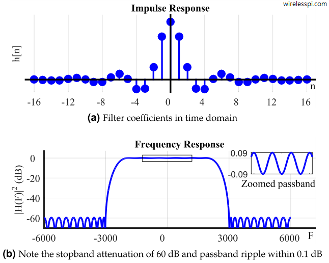
The impulse response $h[n]$ and frequency response $20 \log_{10} H(F)$ of the final filter are drawn in Figure below. Note the stopband attenuation of $60$ dB and passband ripple within $0.1$ dB.

Filtering as Convolution
We also learned above that the higher the number of taps, the more closely the filter follows an expected response (e.g., lowpass, highpass, bandpass, etc.) at a cost of increased computational complexity. Therefore, the defining feature of an FIR filter is the number of coefficients that determines the response length, the number of multipliers and the delay in samples required to compute each output. An FIR filter is built of multipliers and adders. A delay element, which is just a clocked register, is used between coefficients. A single delay element is represented with a $D_1$ symbol. Figure below illustrates a 5-tap FIR filter.
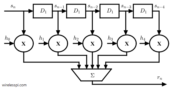
Taking into account the structure in Figure above, this $5$-tap filter output can be mathematically written as
\begin{equation*}
r[n] = h_0 s[n] + h_1 s[n-1] + h_2 s[n-2] + h[3] s[n-3] + h[4] s[n-4]
\end{equation*}
For a general FIR filter of length $N$,
\begin{equation}\label{eqIntroductionFIRFilter}
r[n] = \sum \limits _{m=0} ^{N-1} h[m] s[n-m]
\end{equation}
If this equation sounds familiar to you, you guessed it right. Compare it with the convolution equation, and this is nothing but a convolution between the input signal and the filter coefficients. Just like convolution, at each clock cycle, samples from input data and filter taps are cross-multiplied and the outputs of all multipliers are added to form a single output for that clock cycle. On the next clock cycle, the input data samples are shifted right by $1$ relative to filter taps, and the process continues.
Group Delay
Due to convolution, the length of the output signal $r[n]$ is given as in the article on convolution, which is repeated below.
\begin{equation*}
\text{Length}\{r[n]\} = \text{Length}\{s[n]\} + \text{Length}\{h[n]\} – 1
\end{equation*}
which is longer than the input by $\text{length}\{h[n]\} – 1$ samples. We can say that every FIR filter causes the output signal to be delayed by a number of samples given by
\begin{equation}\label{eqIntroductionFIRDelay}
D = \frac{\text{Length}\{h[n]\} – 1}{2}
\end{equation}
This is known as the group delay of the filter. As a result, $D$ samples of the output at the start — when the filter response is moving into the input sequence — can be discarded. Similarly, the last $D$ samples — when the filter is moving out of the input sequence — can be discarded as well.
Maintaining an exact linear phase in an FIR filter is a straightforward task (but not in general filter design) as follows. Assume that an FIR filter with an odd length has symmetric coefficients.
- Symmetry in coefficients implies that for each sample at time $n_0$, there is a similar sample at time $-n_0$, as the signal is centered at $0$.
- These two samples are two impulses in time domain which form a real sinusoid in frequency domain that represents the spectral amplitude with zero phase.
- Therefore, the only phase comes from the delay that arises from shifting the first sample of the impulse response to time $0$. A shift in time implies a linear phase.
This is why you will usually see a symmetric impulse response of the FIR filters and this is one of the main reasons for widespread use of FIR filters in DSP applications. You can also read a detailed comparison of FIR and IIR (Infinite Impulse Response) filters.