Interpolation in Digital Communication Receivers

Timing synchronization in a digital receiver is about finding the right symbol peak and the symbol rate at which digital samples are taken for decisions purpose in a constellation diagram. In general, interpolation is the process of reproducing a missing sample at a desired location. In digital and wireless communications, the role of interpolation can be explained as follows.

Background

Imagine a Tx signal constructed from the upsampled and pulse shaped modulation symbols. The job of the Rx is to sample this waveform at optimal intervals, i.e., exactly at the middle of the eye diagram. In other words, the Rx only needs one sample per symbol taken at ISI-free locations $T_M$ seconds apart, or $nT_S = mT_M+\epsilon _\Delta$ where $\epsilon _\Delta$ is the original timing phase offset.

However, the sampling clock at the Rx that drives the Analog to Digital Converter (ADC) is often completely unrelated to the clock at the Tx that generated the Tx waveform. Therefore, it is not necessary (and in fact almost impossible) to have samples at the output of the Rx ADC which coincide exactly with the optimal instants.

While timing error detectors provide us with an estimate of timing offset $\hat \epsilon _\Delta$, the timing loop itself is not capable of restoring the signal value at $mT_M+\hat \epsilon _\Delta$. This is the job of the interpolator which in that sense is equivalent to a de-rotation block found in a Phase Locked Loop (PLL). Restoring the phase was a straightforward task where one just needs to de-rotate (clockwise rotation) the signal samples by a given angle. Here, we need a re-computation of the signal values at optimal instants (maximum eye opening).

Next, we discuss how to accomplish the task of interpolating the matched filter output from a set of given samples (usually two or four). The discussion on interpolation and interpolation control is mainly based on Ref. [1] by F. M. Gardner.

Problem Definition

At the output of the matched filter, the samples are available at sample rate $F_S$. A new value needs to be computed between $z(nT_S)$ and $z((n+1)T_S$ at a location $\mu_m T_S$, where $\mu_m$ is the fractional interval during symbol number $m$ that in a TLL targets the maximum eye opening, i.e., at a location
$$\begin{equation*} t = nT_S+\mu_m T_S \end{equation*}$$

Why not just denote this fraction interval as $\mu$? Because this fraction keeps on updating for each symbol $m$ according to the Timing Error Detector (TED) output. Keep in mind that $\mu_m$ is not the TED output $e_D[m]$ since a TED in general sets the direction and magnitude to shift the next sampling interval so as to recursively approach the actual timing phase offset $\epsilon _\Delta$. Moreover, the TED output is filtered by the loop filter to generate the signal $e_F[n]$. This signal is utilized by an interpolator control block to produce the fractional interval $\mu_m$ that informs the interpolator to compute an interpolant at instant $nT_S+\mu_m T_S$. Gradually, the fractional interval $\mu_m$ converges towards the actual timing offset $\epsilon _\Delta$.

Piecewise Polynomial Interpolation

In interpolation using a polynomial, the sample at $nT_S+\mu_m T_S$ is computed through the help of the neighbouring samples. Since this process is performed for each interpolant separately in a timing loop, it is actually known as piecewise polynomial interpolation.

First, consider that the matched filter output $z(nT_S)$ is assumed to have an underlying continuous-time waveform $z(t)$ as
$$\begin{equation}\label{eqTimingSyncPolynomialInterpolation1} z(t) \approx c_p t^p + c_{p-1}t^{p-1} + \cdots + c_1 t + c_0 \end{equation}$$

where $p$ is the degree of the polynomial. Obviously, for the sample value at a time $nT_S+\mu_m T_S$, the above equation can be written as
$$\begin{align} z(nT_S+\mu_m T_S) &\approx c_p (nT_S+\mu_m T_S)^p + c_{p-1}(nT_S+\mu_m T_S)^{p-1} +\nonumber\\ &\hspace{1.5in} \cdots + c_1 (nT_S+\mu_m T_S) + c_0\label{eqTimingSyncPolynomialInterpolation2} \end{align}$$

We consider an implementation through a Finite Impulse Response (FIR) filter for three special cases here, linear interpolation ($p=1$), quadratic interpolation ($p=2$) and cubic interpolation ($p=3$).

Linear Interpolation, $p=1$

Plugging $p=1$ in Eq ($\ref{eqTimingSyncPolynomialInterpolation1}$), we get
$$\begin{equation*} z(t) \approx c_1 t + c_0 \end{equation*}$$

To find the values of two coefficients $c_1$ and $c_0$, we need two equations. Therefore, we employ two neighbouring samples $z(nT_S)$ and $z((n+1)T_S)$ such that
$$\begin{align*} z(nT_S) &= c_1 nT_S+c_0 \\ z((n+1)T_S) &= c_1 (n+1)T_S + c_0 \end{align*}$$

Subtracting the former equation from the latter,
$$\begin{align*} z((n+1)T_S) – z(nT_S) &= c_1(nT_S+T_S-nT_S) \\ c_1 &= \frac{z((n+1)T_S)-z(nT_S)}{T_S} \end{align*}$$

The coefficient $c_0$ is thus given by
$$\begin{align*} c_0 &= z(nT_S) – c_1 nT_S\\ &=z(nT_S) – \frac{z((n+1)T_S)-z(nT_S)}{T_S}nT_S \\ &= (1+n)z(nT_S) – n z((n+1)T_S) \end{align*}$$

Having known $c_0$ and $c_1$, we can now compute the interpolant $z(nT_S+\mu_m T_S)$. Plugging $p=1$ in Eq ($\ref{eqTimingSyncPolynomialInterpolation2}$),
$$\begin{equation*} z(nT_S+\mu_m T_S) \approx c_1 (nT_S+\mu_m T_S) + c_0 \end{equation*}$$

which yields
$$\begin{align*} z(nT_S+\mu_m T_S) &= \frac{z((n+1)T_S)-z(nT_S)}{T_S}(nT_S+\mu_m T_S) + \\ &\hspace{1.5in}(1+n)z(nT_S) – n z((n+1)T_S)\\ &= \mu_m z((n+1)T_S) -\mu_m z(nT_S) + z(nT_S) \end{align*}$$

The expression for the linear interpolator is thus written as

An example of linear interpolation is drawn in the figure below. Observe how the interpolant is computed as a point at the desired location by connecting the two neighbouring samples through a straight line.

From Eq ($\ref{eqTimingSyncLinearInterpolation}$), observe that the interpolant $z(nT_S+\mu_m T_S)$ is a linear combination of $z(nT_S)$ and $z((n+1)T_S)$. Therefore, it can be thought of as their convolution with a filter $h_1[n]$.
$$\begin{align*} z(nT_S+\mu_m T_S) &= \mu_m z((n+1)T_S) + (1-\mu_m)z(nT_S)\\ &= h_1[-1] z((n+1)T_S) + h_1[0] z(nT_S) \\ &= \sum \limits _{i=-1} ^0 h_1[i] z((n-i)T_S) \end{align*}$$

The filter coefficients are thus given by
$$\begin{equation} \begin{aligned} h_1[-1] &= \mu_m \\ h_1[0] &= 1-\mu_m \end{aligned} \end{equation}\label{eqTimingSyncLinearFilter}$$

where the subscript $1$ denotes linear interpolation ($p=1$). Furthermore, the index $-1$ in $h[-1]$ signifies the fact that we are employing $z((n+1)T_S)$ instead of $z((n-1)T_S)$.

Quadratic Interpolation, $p=2$

Plugging $p=2$ in Eq ($\ref{eqTimingSyncPolynomialInterpolation1}$), we get
$$\begin{equation*} z(t) \approx c_2 t^2 + c_1 t + c_0 \end{equation*}$$

Therefore,
$$\begin{equation*} z(nT_S+\mu_m T_S) \approx c_2 (nT_S+\mu_m T_S)^2 + c_1 (nT_S+\mu_m T_S) + c_0 \end{equation*}$$

To find the values of three coefficients $c_2$, $c_1$ and $c_0$, we need only three equations and hence just three samples out of the matched filter, namely $z((n-1)T_S)$, $z(nT_S)$ and $z((n+1)T_S)$. However, if we take that route, there will be no middle two samples between which the interpolant can be constructed. Then, the FIR filter will not be symmetric with respect to $\mu_m = 1/2$. As mentioned above, an even number of samples are required to ensure a linear phase response of the FIR filter. Consequently, an extra fourth sample is used for quadratic interpolation.

Skipping the derivation, the desired interpolant can again be written as the output of a filter as
$$\begin{align*} z(nT_S+\mu_m T_S) &= h_2[-2] z((n+2)T_S) + h_2[-1] z((n+1)T_S) + \\ &\hspace{1.3in}h_2[0] z(nT_S) + h_2[1] z((n-1)T_S)\\ &= \sum \limits _{i=-2} ^1 h_2[i] z((n-i)T_S) \end{align*}$$

where the filter coefficients are given by
$$\begin{align} \begin{aligned}\label{eqTimingSyncQuadraticFilter} h_2[-2] &= \beta \mu_m^2 – \beta \mu_m \\ h_2[-1] &= -\beta \mu_m^2 + (1+\beta)\mu_m\\ h_2[0] &= -\beta \mu_m^2 – (1-\beta)\mu_m+1\\ h_2[1] &= \beta \mu_m^2 -\beta \mu_m \end{aligned} \end{align}$$

In the above equations, the subscript $2$ denotes quadratic interpolation ($p=2$) and $\beta$ is an additional parameter to choose due to an extra sample being used. A value of $\beta=0.5$ is usually used to reduce the hardware complexity as multiplication and division by a factor of $2$ can be implemented by simple left and right shifts of the contents of a register. An example of quadratic interpolation is drawn in the figure below.

Notice the parabolic overshoots emerging from the sample values due to piecewise computation, generating vastly improved results without expending significant computational resources. See the Farrow structure for a simplified implementation of a cubic interpolator.

Ideal Interpolation, $p=\infty$

To unify the above findings, consider the general convolution equation out of an interpolating filter with degree $p$.
$$\begin{equation*} z(nT_S+\mu_m T_S) = \sum \limits _{i=-2} ^1 h_p[i] z((n-i)T_S) \end{equation*}$$

The filter coefficients for $p=1$ and $2$ were derived before. Something interesting happens when we vary $\mu_m$ from $0$ to $1$,
$$\begin{equation*} \mu_m: ~0 ~\rightarrow ~ 1 \end{equation*}$$

and plot the filter coefficients as a function of $\mu_m$. For example, for $p=1$,
$$\begin{align*} h_1[-1] &= \mu_m \\ h_1[0] &= 1-\mu_m \end{align*}$$

So for $t/T_S$ between $-1$ to $0$ (which is the same as $t$ from $-T_S$ to $0$), the plot of $h_1(-1+\mu_m)$ is $\mu_m$ which goes from $0$ to $1$.
$$\begin{equation*} h_1(-1+\mu_m) :~ 0 ~\rightarrow ~ 1 \end{equation*}$$

Here, $h_1(-1+\mu_m)$ is the interpolated version of the discrete-time impulse response of the filter $h_1[n]$. Similarly, for $t/T_S$ between $0$ to $1$ (which is the same as $t$ from $0$ to $T_S$), the plot of $h_1(0+\mu_m)$ is $1-\mu_m$ which goes from $1$ to $0$.
$$\begin{equation*} h_1(0+\mu_m) :~ 1 ~\rightarrow ~ 0 \end{equation*}$$

In general, we can draw the impulse response $h_1(n+\mu_m)$ from $-1$ to $1$. This is because the filter coefficients are at locations $-1$ and $0$ while $\mu_m$ ranges from $0$ to $1$.

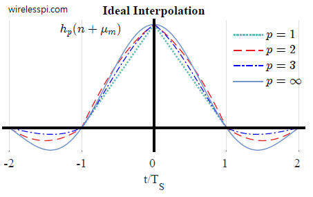
A similar procedure is followed for $h_2(n+\mu_m)$ and $h_3(n+\mu_m)$ between $-2$ and $2$. The results are plotted in the figure below in an increasing order. Notice that as the degree $p$ of the polynomial increases, the filter becomes closer in shape to a sinc signal.

Now this is the most beautiful part: Why did the sinc signal appear here? Recall from sample rate conversion that after inserting zeros during an upsampling process, a lowpass filter is employed to reject the spectral replicas leaving only the central spectrum. In time domain, this filtering has the effect of interpolating between the samples because multiplication with a rectangular filter in frequency domain is equivalent to convolving with a sinc function in time domain. This sinc function has integer spaced zero crossings due to which its convolution with a sampled signal creates the output exactly as the input at discrete-time intervals and a combination of those samples in between. That is why as we increase the degree $p$ of our polynomial approximation towards $p=\infty$, our filter impulse response approaches a sinc signal.

References

[1] F. M. Gardner, Interpolation in Digital Modems, Part I and II, IEEE Transactions on Communications, 1993.