In digital logic, a stream of 1s and 0s forms a sequence of rectangular pulses, which can be easily identified at the receiver side by a threshold. In time domain, everything looks nice and perfect.

Let us investigate the system characteristics in frequency domain. In a Pulse Amplitude Modulation (PAM) system, the main component that defines the spectral contents of the signal is the pulse shape $p(nT_S)$ at the Tx. We start with our attention towards a simple rectangular pulse shape.

Here is a brief outline of what we cover in this article.

Table of Contents

Let us start with the spectrum of a rectangular pulse.

Spectrum of a Rectangular Pulse

In time domain, a rectangular pulse has a clear benefit that Tx symbols do not naturally invade into each other’s territory. In case there are no reflections or dispersions in the channel, there are no adjacent symbols interfering into each other at the Rx as well — a phenomenon called Inter-Symbol Interference (ISI). ISI simplifies the detector in Rx design because everything related to a particular $m$th symbol remains within the symbol interval $(m-1)T_M \le t \le mT_M$. Or in other words, what happens in a symbol duration stays within that symbol duration.

As for the frequency domain, we derived an analytical expression for the DFT of a rectangular sequence in the article on DFT examples as
\begin{equation*}
|P_{\text{rect}}[k]| = \frac{\sin \pi L k/N}{\sin \pi k/N}
\end{equation*}
In the graph of this sinc function, nulls should occur wherever the numerator is zero, except at $k/N=0$ where the peak exists. Now $\sin(\cdot)=0$ when its argument is an integer multiple of $\pi$. Thus, equating the argument of the numerator to $\pi$ returns the first null position.
\begin{align*}
\pi L \left(\frac{k}{N}\right)_{\text{null}} = \pi \quad \quad \Rightarrow \quad \quad \left(\frac{k}{N}\right)_{\text{null}} = \frac{1}{L}
\end{align*}
Thus, the positions of nulls are $\pm 1/L, \pm 2/L, \pm 3/L, \cdots$ with respect to discrete frequency $k/N$. In Hz, with $F_S=L\cdot R_M$, the null positions are $\pm R_M, \pm 2R_M$, $\pm 3R_M$, $\cdots$ because
\begin{equation*}
F_{\text{null}} = F_S \cdot \left(\frac{k}{N}\right)_{\text{null}} = F_S\cdot\frac{1}{L} = R_M
\end{equation*}
Finally, the range is
\begin{align*}
-0.5F_S = -0.5 L\cdot R_M \le F < +0.5 L\cdot R_M = +0.5 F_S \end{align*} which for $L=8$ samples/symbol produces \begin{align*} -4 R_M \le F < +4 R_M \end{align*} The spectrum of a rectangular pulse shape shows these deductions in Figure below.

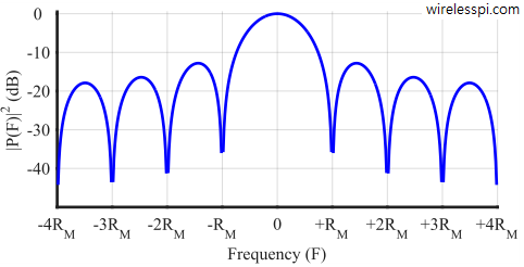
A great disadvantage of a rectangular pulse shape is now visible: the sidelobe level is just $-13$ dB below the mainlobe, a very high value. Furthermore, the subsequent sidelobes are not decaying fast enough. If there is a communications link which occupies the drawn spectrum and the neighboring spectrum is allocated to someone else, then there will be a lot of interference between the two parties due to their sidelobe energies interfering with each other.

Just like real estate, radio spectrum is a very precious resource and must be utilized judiciously. This is why there are spectrum regulatory authorities in every country who impose strict restrictions to comply with a spectral mask. Even for wired channels, there is always a natural bandwidth of the medium (copper wire, coaxial cable, optical fiber) that imposes upper limits on its utilization.

Not only that a rectangular pulse shape is a poor choice due to its large spectral occupancy, another side effect of having a wider bandwidth pulse shape is that the matched filter at the Rx also has a similar bandwidth. Viewed in frequency domain, the larger the bandwidth of the Rx filter, the more noise and interference it allows to enter the system.

Reducing the bandwidth

Having known the disadvantages of a rectangular pulse shape, a superior pulse shaping filter needs to be looked for that should help in placing multiple channels adjacent to each other while minimizing inter-channel interference between them as well as noise bandwidth at the Rx. However, such advantages should not come at a price of introducing ISI in the system.

Nyquist No-ISI Criterion in Time Domain

To get that superior pulse shape, we trace the following sequence of steps through the help of Figure below that plots the auto-correlation $r_p(nT_S)$ of both a rectangular and a conceptual pulse shape. Auto-correlation of a pulse shape was defined earlier as
\begin{equation*}
r_p(nT_S) = \sum \limits _i p(iT_S) p(iT_S – nT_S)
\end{equation*}
and plots are shown in continuous-time to make the related steps below more understandable.

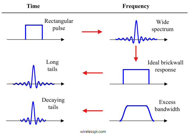
• Remember that we discussed that signals that are narrow in time domain are wide in frequency domain, and vice versa. Accordingly, a consequence of narrow time span of the pulse shape is that it gets expanded in frequency. That is why a rectangular pulse has a large bandwidth. To decrease the bandwidth, the length of the pulse shape needs to be extended in time domain — much more than a single symbol duration $T_M$.
• The effect of extending the length of the pulse shape is that every symbol now interferes with a number of symbols occurring both before and after that symbol. The dreaded ISI appears! Assuming a usual even shaped pulse, every symbol contributes towards ISI in symbols towards its left and symbols towards its right on time axis.
• To strike peace with this ISI, we exploit a key property of digital communication waveforms explained before: the critical samples at the output of matched filter occur at the end of integer multiples of symbol duration $T_M$. For symbol detection, only these $T_M$-spaced samples are needed and the rest can be discarded. This is what we saw at the output of the downsampler in PAM block diagram.

  If all but one sample during each symbol interval $T_M$ are discarded, they can be assigned any value without any effect on the detector output. These are the “don’t care” samples we give up for ISI to play with in the expectation that we get to shape our desired spectrum in return, and with the result that our desired $T_M$-spaced samples remain intact. Keep in mind that we are talking about the output of the matched filter — and hence auto-correlation of the pulse shape — here. The reason is to elaborate the nature of signal that is eventually downsampled to yield symbol estimates. The actual pulse shape will be extracted from this auto-correlation, as we will shortly see.

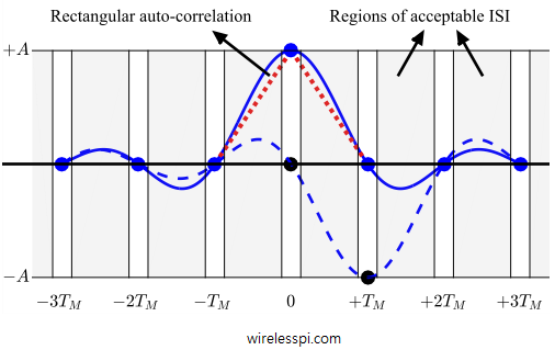
• In the light of above discussion, three pulse shape auto-correlations are illustrated in the Figure above.
  1. A rectangular pulse shape has a duration of $T_M$ seconds, or $L$ samples. Hence, its auto-correlation extending over $2T_M$ seconds. Notice that it has a maximum value at the desired current sampling instant and zero for adjacent two symbols. The time span, however, is too short giving rise to an unreasonably large spectrum.
  2. A pulse shape auto-correlation that is expanded over many symbols is shown in blue curve, where it is scaled by a symbol $+A$. Note that at all the sampling instants (integer multiples of $T_M$), the effect of this particular symbol is zero. We intend to assign values to its “don’t care” samples in shaded regions to achieve a compact spectrum.
  3. An adjacent symbol $-A$ scales the same pulse shape at time $T_M$. Observe the same zero-ISI effect on the current symbol at time $0$ and on all other symbols.

Not shown in the above figure are all other symbols shaped by pulses at $2T_M$, $3T_M$, and so on. But it is clear that sum total of ISI from all adjacent symbols is zero at sampling instant of every single symbol. For a concrete formulation of this zero-ISI criterion, we turn towards its mathematical foundation.

Just as in the case of rectangular pulse in the article on Pulse Amplitude Modulation (PAM), the input signal is
\begin{equation*}
s(nT_S) = \sum _{i} a[i] p(nT_S-iT_M)
\end{equation*}

Although this equation was derived for a pulse with duration $T_M$, it is also true for longer pulses because
\begin{align*}
\sum _{i} a[i] p(nT_S-iT_M) &= a[0]p(nT_S) + a[1] p (nT_S-T_M) ~+ \\
& \hspace{2in} a[2] p(nT_S – 2T_M) + \cdots \\
&= \Big( a[0] \delta[nT_S] + a[1] \delta[nT_S-T_M] ~+ \\
& \hspace{1.3in} a[2] \delta [nT_S-2T_M] + \cdots \Big) * p(nT_S)
\end{align*}
This is because convolution between any signal and a unit impulse results in the same signal. Therefore, even for longer pulses, scaling each individual symbol with its own pulse shape is equivalent to convolution of symbol stream with a pulse shaping filter.

When this signal is input to matched filter $h(nT_S) = p(-nT_S)$, the output is written as
\begin{align*}
z(nT_S) &= \Big( \sum \limits _i a[i] p(nT_S – iT_M)\Big) * p(-nT_S) \\
&= \sum \limits _i a[i] r_p(nT_S – iT_M)
\end{align*}

To generate symbol decisions, $T_M$-spaced samples of the matched filter output at $n = mL = mT_M/T_S$ are
\begin{align}
z(mT_M) &= z(nT_S) \bigg| _{n = mL = mT_M/T_S} \nonumber \\
&= \sum \limits _i a[i] r_p(mT_M – iT_M) = \sum \limits _i a[i] r_p\{(m-i)T_M\} \nonumber \\
&= \underbrace{a[m] r_p(0T_M)}_{\text{current symbol}} + \underbrace{\sum \nolimits _{i \neq m} a[i] r_p\{(m-i)T_M\}}_{\text{ISI}} \label{eqCommSystemRxSymbol}
\end{align}

In the above equation, the first term is the currently desired symbol and the second term is inter-symbol interference (ISI). It is obvious that ISI can be zero if the pulse auto-correlation satisfies the condition
\begin{equation}\label{eqCommSystemNoISITime}
r_p(mT_M) = \left\{ \begin{array}{l}
1, \quad m = 0 \\
0, \quad m \neq 0 \\
\end{array} \right.
\end{equation}

This is Nyquist no-ISI criterion in time domain — a mathematical expression of the same concept we explained above: to obtain zero ISI, the pulse auto-correlation should pass through zero for all integer multiples of $T_M$ before and after the current symbol.

When Nyquist no-ISI criterion in time domain is satisfied, plugging Eq \eqref{eqCommSystemNoISITime} into Eq \eqref{eqCommSystemRxSymbol} gives

i.e., the downsampled matched filter output maps back to the Tx symbol in the absence of noise. This is the crux of digital communications theory.

Nyquist no-ISI Criterion in Frequency Domain

Throughout the article, we have been avoiding complicated mathematical derivations. We will do the same here and instead of proving Nyquist no-ISI theorem which connects time and frequency domain properties of pulse auto-correlation, we again take the intuitive route.

As long as we operate at a sample rate $F_S$, the spectral replicas are spaced at $F_S = LR_M$ apart. But since we downsample $r_p(nT_S)$ by $L = T_M/T_S$ to get $r_p(mT_M)$, our sample rate changes from $F_S$ at the output of matched filter to $R_M$ after the downsampler. To see what happens in frequency domain, observe that

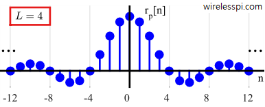
• In discrete domain, $r_p(mT_M)$ in Eq \eqref{eqCommSystemNoISITime} is nothing but a single impulse at time $0$. This can be seen as the blue dots in first part of Figure below. Hence, its DFT is an all-ones rectangular sequence in frequency domain, which was derived in the article on DFT examples as
  \begin{equation*}
  R_p[k] = 1
  \end{equation*}
• Moreover, we know from the post on sample rate conversion that a consequence of downsampling by $L$ is appearance of new spectral aliases $R_M$ apart from each other.

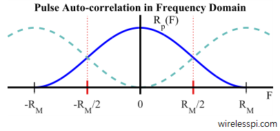
Combining the above two facts produces second part of Figure below illustrating this relationship between symbol-spaced pulse auto-correlation and its Fourier transform.

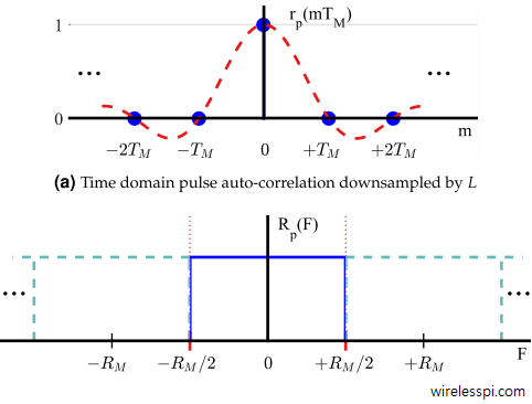
We can also see that the signal bandwidth $B$ in this particular case is (never confuse a rectangular pulse shape in time domain with a pulse auto-correlation that is a rectangle in frequency domain)
\begin{equation*}
B = 0.5R_M
\end{equation*}
This is the maximum bandwidth after which aliasing will occur from spectral replicas. This also sets the fundamental limit between the bandwidth $B$ and symbol rate $R_M$ as

Hence, with zero ISI, a maximum symbol rate $R_M$ equal to $2B$ symbols/second can be supported within a bandwidth $B$.

Remember that the point of this whole exercise was to limit the enormous bandwidth occupied by a time domain rectangular pulse. In other words, the quest is to design a pulse shape such that it complies with the spectral mask within a channel bandwidth $B$. Nyquist no-ISI criterion in frequency domain helps here.

Nyquist showed that a necessary and sufficient condition for zero ISI condition of Eq \eqref{eqCommSystemNoISITime} is that the Fourier transform $R_p(F)$ of the pulse auto-correlation satisfies the condition
\begin{align}
\sum \limits _{i=-\infty} ^{\infty} R_p(F + iR_M) &= \cdots + R_p(F + 2R_M) + R_p(F + R_M) + \nonumber\\
&\hspace{0.8in} R_p(F) + R_p(F – R_M) + R_p(F – 2R_M) + \cdots \nonumber \\
&= \text{constant} \label{eqCommSystemNoISIFreq}
\end{align}

Its proof is not much complicated but we skip it anyway and rely on intuition. A hint about Nyquist no-ISI criterion in frequency domain comes from the Figure above: the spectrum of the pulse auto-correlation should be a constant. All it says is that for the DFT of pulse auto-correlation,

• Draw the primary spectrum $R_p(F)$ whose range is $-0.5F_S \le F < +0.5F_S$.
• Draw its shifted replicas at frequencies $\pm R_M$. Repeat the same for all integer multiples of $\pm R_M$ from $-\infty$ to $+\infty$.
• Add all these replicas together.
• If this sum results in a constant, only then the time domain pulse auto-correlation will satisfy the no-ISI condition Eq \eqref{eqCommSystemNoISITime}.

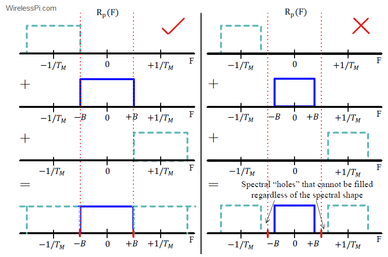
Figure above shows two spectra, one of which satisfies the Nyquist no-ISI criterion while the other does not. The spectrum on the left is constant because the bandwidth is as wide as allowed by sampling theorem (which is $B_{\text{max}}=0.5R_M$ for sample rate $R_M$). This not only avoids aliasing but owing to a flat spectrum within $-0.5R_M$ $\le F <$ $+0.5R_M$ produces a flat spectrum in range $-1.5R_M$ $\le F <$ $-0.5R_M$, $+0.5R_M$ $\le F <$ $+1.5R_M$, and so on. Consequently, the cumulative spectrum as in Eq \eqref{eqCommSystemNoISIFreq} is a constant function of frequency from $-\infty$ to $+\infty$. Interestingly, this maximum bandwidth $0.5R_M$ allowed by sampling theorem is also the minimum bandwidth allowed by Nyquist no-ISI criterion in frequency domain. Any smaller than this, and it becomes impossible to obtain an overall flat spectrum. That is shown on the right of Figure above where there are spectral “holes” that cannot be filled regardless of the spectral shape.

Coefficients of an Ideal Pulse Auto-correlation

Above, we said that a filter whose impulse response coefficients satisfy Nyquist no-ISI criterion is a Nyquist filter, which is actually the auto-correlation $r_p(nT_S)$ of the underlying pulse shape. From Figure above and the discussion in the last section, we find our ideal Nyquist filter: a pulse auto-correlation $r_p(nT_S)$ whose spectrum $R_p(F)$ is a rectangle from $-0.5R_M$ to $+0.5R_M$.

To derive the time domain representation of such a filter, remember that a rectangle in frequency domain is a sinc in time domain due to time frequency duality. This rectangle covers the entire continuous frequency range from $F=-0.5R_M$ to $+0.5R_M$ (or discrete frequency range $k/N=-0.5$ to $+0.5$) yielding $L = N$ in DFT of a rectangular signal (this $L$ is not samples/symbol, just the sequence length in that equation). There is a scaling factor of $1/N$, furthermore, from the definition of iDFT. Combining these facts,
\begin{equation*}
s[n] = \frac{1}{N} \frac{\sin \pi n}{\sin \pi n/N}
\end{equation*}
For our purpose with a sample rate of $R_M$ so far,
\begin{equation*}
r_p[m] = \frac{1}{N} \frac{\sin \pi m}{\sin \pi m/N}
\end{equation*}
It satisfies Eq \eqref{eqCommSystemNoISITime} because it is equal to $1$ at $m=0$ and zero for $m \neq 0$ and shown as blue dots in the Figure before.

Using the identity $\sin \theta \approx \theta$ for small $\theta$, the term in the denominator is quite small as compared to numerator due to division by $N$. Then, the above equation can be written as
\begin{equation*}
r_p[m] \approx \frac{1}{N} \frac{\sin \pi m}{\pi m/N} = \frac{\sin \pi m}{\pi m}
\end{equation*}
This is the time domain waveform sampled at rate $R_M$. As we are interested in time domain coefficients $r_p[n]$ of this ideal pulse auto-correlation, we sample the waveform at rate $F_S = L\cdot R_M$ instead of just $R_M$, an increase by a factor of $L$. Correspondingly, a decrease in sample time yields
\begin{equation}\label{eqCommSystemRectangleSinc}
r_p[n] = \frac{\sin \pi n/L}{\pi n/L}
\end{equation}
These are the coefficients of our ideal pulse auto-correlation, which extends from $-\infty$ to $+\infty$ in time domain as shown in Figure below.

There are two main problems with this ideal pulse auto-correlation, both arising due to a very slow rate of decay for the tail.

[Truncation Error] Any practical system cannot use a filter with an infinite number of coefficients like the one shown in the figure of coefficients for an ideal pulse auto-correlation. Hence, the filter impulse response must be truncated at a few symbols to the left and a few symbols to the right of the current symbol. To ensure that this truncated filter closely approximates the ideal impulse response, only very small values can be ignored. That generates a large filter length $N$.

[Timing Errors] We know that optimal timing instant coincides with symbol boundaries. Timing synchronization block in a Rx is responsible for extracting this symbol-aligned clock. However, even a small error in timing synchronization output causes a significant increase in ISI due to large value of samples at the tail interacting with neighbouring modulated pulses. The quicker the tail decay is, the lesser the errors arising from timing jitter when sampling adjacent pulses.

To address these issues, we take the reverse route now. We started with the aim of reducing the bandwidth of a rectangular pulse shape. We found an ideal pulse auto-correlation with a rectangular spectrum that satisfies Nyquist no-ISI criterion. To overcome the limitations in time domain associated with it, we seek to trade-off some bandwidth with desirable time domain behaviour.

Raised Cosine (RC) Filter

Remember that we observed regions of acceptable ISI in auto-correlation figure of a conceptual pulse and deduced that these “don’t care” samples can be given up for ISI to play with in the expectation that we get to shape our desired spectrum in return, while our $T_M$-spaced samples remain intact.

We have found the restriction to be a flat spectrum across the whole frequency range. The relaxation is that how this spectrum becomes flat is a matter of no concern. The actual spectral shape is a “don’t care” case, as long as the sum of all shifted replicas is flat.

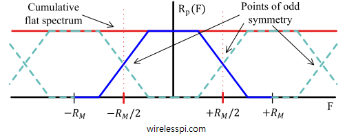
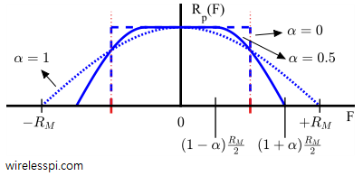
It is clear that we cannot reduce the bandwidth below the fundamental limit $0.5R_M$. The only way to alter the spectral shape is by expanding the bandwidth beyond $0.5R_M$ in such a way that the sum total of the replicas again becomes flat. For this purpose, an odd symmetry around the point $0.5R_M$ is required. The advantage of such odd symmetry is that the spectral magnitudes before and after $0.5R_M$ are $180^\circ$ rotated versions of each other. In other words, the spectral copies at $\pm R_M$ fold around $\pm 0.5R_M$ into the original bandwidth. That supplies the additional amplitude required to bring the spectrum in a flat shape, as illustrated in Figure below.

Higher frequency components of a signal arise from abrupt changes in time domain, which was the reason of large spectral occupancy of a rectangular pulse shape. Similarly, long tails in a time domain signal arise from abrupt transition in the flat spectrum. Also recall from the post on FIR filters that the length of an FIR filter depends on its transition bandwidth.

Having located the abrupt transition bandwidth around $\pm 0.5R_M$ as the root cause, we can extend the bandwidth of the pulse auto-correlation in any shape as long as it has odd symmetry around the points $\pm 0.5R_M$. The purpose is to smooth out its spectrum.

The smoothest spectral shape one can imagine is a sinusoid. If such a spectral taper is convolved with the ideal rectangular spectrum, the discontinuity in the spectrum can be removed. Since a half-cosine is an even symmetric shape, it is shown to be convolved with the rectangular spectrum in Figure below. The width of the half-cosine is $\alpha R_M$ where $0 \le \alpha \le 1$ which forms the transition bandwidth of the resultant spectrum and its even symmetric shape preserves the odd symmetry around $\pm 0.5R_M$. As a consequence of this odd symmetry, this is also a Nyquist filter. The resultant spectrum out of this convolution is discussed soon.

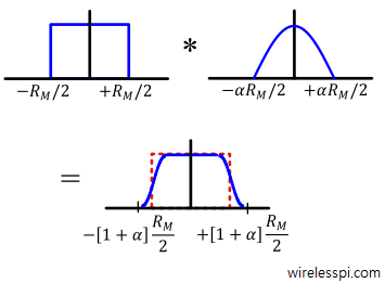
It can be observed that the effect of spectral convolution is an increase in bandwidth from $0.5R_M$ to $0.5(1+\alpha) R_M$. Since $\alpha$ specifies the bandwidth beyond the minimum bandwidth $0.5R_M$ (Nyquist frequency or folding frequency), it is called excess bandwidth or roll-off factor. For example, when $\alpha=0.25$, the total bandwidth is $25 \%$ more than the minimum and when $\alpha=1$, the total bandwidth is exactly $100 \%$ more than, or twice, the minimum. Typical values of $\alpha$ range from $0.1$ to $0.3$. Excess bandwidth of roll-off factor also plays a major role in achieving timing synchronization in digital communication systems.

In time domain, this is equivalent to product of a sinc signal with an even signal of time (since the spectrum is real and even, the time domain signal is also real and even). The sinc signal guarantees the zero crossings as they cannot be moved by multiplication, and the even signal dampens the long tails in time. The higher the bandwidth, the narrower this signal is and hence faster the decay.

First, consider $\alpha = 1$, the widest bandwidth case. Here, a rectangle of spectral width $R_M$ gets convolved with a half-cosine of width $R_M$. The convolution of the resultant spectrum again generates a cosine shape from $F=-R_M$ to $+R_M$ for a total width of $2R_M$. This is plotted in Figure below, where smooth frequency transition can be seen with an odd symmetry around $\pm 0.5R_M$. It is commonly known as a Raised Cosine (RC) filter (Raised Cosine (RC) filter has nothing to do with an RC circuit consisting of a resistance and a capacitor). The name raised cosine comes from the fact that {the transition bandwidth of the spectrum consists of a cosine raised by a constant to make it non-negative, see Eq \eqref{eqCommSystemRaisedCosineAlpha1} and Eq \eqref{eqCommSystemRaisedCosineFreq} later.

Let us explore its mathematical expression. Due to the way it is usually written in literature, the formula looks more complicated that it actually is. Recall that a sinusoid in time domain is written as
\begin{equation*}
s(t) = \cos (2\pi \underbrace{F} _{=1/T,~\text{inverse period}} ~ \underbrace{t} _{\text{independent variable}}
\end{equation*}

A frequency domain sinusoid will just interchange these roles, with inverse period and independent variable defined in terms of frequency. A cosine from $F=-R_M$ to $+R_M$ implies that the period in frequency is $2R_M$ (the inverse of which is $T_M/2$)). Also, it is raised by a constant $1$ to make it non-negative and scaled by $0.5$ to get a unity gain. Thus, the expression for this cosine spectrum on the positive half is given as
\begin{align*}
R_p(F) &= 0.5 + 0.5 \cos ( 2 \pi \underbrace{1/2R_M} _{\text{inverse period}} ~\underbrace{F} _{\text{independent variable}} ) \\
&= 0.5 \left[1 + \cos (2 \pi \frac{T_M}{2} F)\right] \quad \quad \quad 0 \le F \le +R_M
\end{align*}

We obtain its time domain expression through the following steps:

• In frequency domain, the constant term and cosine in the above expression do not have a frequency support from $-\infty$ to $\infty$, but only from $-R_M$ to $+R_M$.
• In frequency domain, that is equivalent to multiplication with a rectangular window of the same width.
• Multiplication in frequency domain is convolution in time domain.
• In time domain, the constant term translates to an impulse at time location $0$, and $\cos(\cdot)$ results in two impulses with half that amplitude at time locations (inverse period) $\pm T_M/2$.
• In time domain, the rectangular window of width $2R_M$ in frequency is a sinc signal with zero crossings at integer multiples of $\pm 1/2R_M = \pm T_M/2$.
• Convolution of a signal with an impulse is the signal itself. When convolved with sinc arising from the window, this generates three sinc signals: one at time $0$ while two at time $\pm T_M/2$.

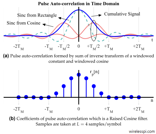
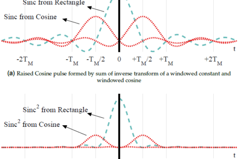
The above sequence of steps result in time domain signal of an extended bandwidth pulse auto-correlation shown in Figure below. The reason of choosing a frequency support $-R_M \le F \le +R_M$ is now clear. With $B = 2R_M$ in frequency, the sinc resulting from cosine adds out of phase at $t = T_M/2$ with the sinc from the constant term. The signs of their tails are opposite to each other and that is what brings down the levels of long tails of an ideal pulse auto-correlation. Furthermore, sincs from both constant term and cosine have zero crossings at integer multiples of $\pm T_M/2$, as marked through the ellipse in the figure. Nevertheless, a time shift of $T_M/2$ for the sinc from cosine causes the cumulative signal to pass through zero at integer multiples of $\pm T_M$. This is how this pulse auto-correlation fulfills the Nyquist no-ISI criterion in time domain. Finally, sampling the pulse auto-correlation at $L=4$ samples/symbol produces the discrete-time coefficients that can be used for pulse shaping in digital domain.

Compare this discrete-time signal with the ideal Nyquist filter in the figure of coefficients for an ideal pulse auto-correlation before. Now we can truncate the filter to a small length without much loss in accuracy. In addition, a sampling time misalignment at the Rx will have a minor influence on the current symbol and not much. Remember that the cost of this relief is the wider bandwidth $2R_M$. Observing this trend, we can think of striking a trade-off between the filter length and bandwidth expansion. The excess bandwidth $\alpha$ comes into play here.

For this purpose, the excess bandwidth $\alpha$ can be reduced from $\alpha=1$ to a lower value. By reducing the bandwidth, the following sequence occurs.

• When $\alpha < 1$, the period in frequency of the half-cosine (on each side of zero) in the Raised Cosine spectrum with excess bandwidth equal to 1 decreases, while still maintaining odd symmetry around $\pm 0.5R_M$.
• As shown in Figure below, a decrease in frequency period results in three distinct regions of the spectrum: a half-cosine in the positive part of spectrum
  \begin{equation*}
  +0.5(1-\alpha)R_M \le F \le +0.5(1+\alpha)R_M,
  \end{equation*}
  a half-cosine in the negative portion of the spectrum
  \begin{equation*}
  -0.5(1+\alpha)R_M \le F \le -0.5(1-\alpha)R_M,
  \end{equation*}
  and a constant term
  \begin{equation*}
  -0.5(1-\alpha)R_M \le F \le +0.5(1-\alpha)R_M.
  \end{equation*}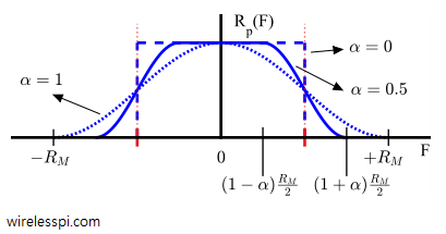

  

  Note that when $\alpha=1$, the bandwidth was $R_M$ which can be written as $0.5(1+1)R_M$. A decrease in $\alpha$ results in new bandwidth $0.5(1+\alpha)R_M$ as drawn in Figure above. Also observe that $\alpha=0$ case coincides with a rectangular spectrum of ideal Nyquist filter. This was the minimum bandwidth allowed by Nyquist no-ISI criterion.

• A decrease in bandwidth results in multiple windowed cosines and a constant. To avoid complication, its detailed analysis is not necessary. We just note that as $\alpha$ gets smaller and smaller, the sincs in time domain resulting from windowed cosine in frequency move away from each other, thus causing less tail suppression as compared to $\alpha =1$ case. In conclusion, the excess bandwidth $\alpha$ gives the system designer a trade-off between reduced bandwidth and time domain tail suppression.

Taking clue from Eq \eqref{eqCommSystemRaisedCosineAlpha1}, the general expression for a Raised Cosine can be written as

\begin{equation}\label{eqCommSystemRaisedCosineFreq}
R_p(F) = \left\{ \begin{array}{l}
1 \hspace{2in} 0 \le |F| \le 0.5(1-\alpha)R_M \\
0.5 \left[1 + \cos \left\{2\pi \frac{T_M}{2\alpha} \left( |F| – (1-\alpha)\frac{R_M}{2}\right)\right\} \right] \\
\hspace{1.29in} 0.5(1-\alpha)R_M \le |F| \le 0.5(1+\alpha)R_M \\
0 \hspace{2.3in} |F| \ge 0.5(1+\alpha)R_M
\end{array} \right.
\end{equation}

The above equations looks intimidating but it is not. There are only three minor differences from Eq \eqref{eqCommSystemRaisedCosineAlpha1}.

1. $T_M/2\alpha$ in the middle term shows a reduction in bandwidth and a spectral shift of cosine center from $F=0$ to $F = 0.5(1-\alpha)R_M$. This is the edge of the passband now and $0.5(1-\alpha)R_M$ is called the passband frequency.
2. The first term is a constant occupying the bandwidth left behind by the half-cosine.
3. The final term shows no bandwidth occupied from $0.5(1+\alpha)R_M$ onwards. This is the start of the stopband and $0.5(1+\alpha)R_M$ is called the stopband frequency.

Now it is clear why an oversampling factor of $L$ samples/symbol – a sampling rate of $L \cdot R_M$ – is used in digital communication systems. Applying sampling theorem to the stopband frequency $0.5(1+\alpha)R_M$, the sampling theorem sets the minimum sampling rate at $(1+\alpha)R_M$.

To obtain its time domain expression, recall from the figure on spectral convolution where we found that the resultant waveform in time domain is equivalent to product of a sinc signal with an even signal of time.

\begin{align}\label{eqCommSystemRaisedCosineTime}
r_p [n] = \frac{1}{L}\cdot \frac{\sin(\pi n/L)}{\pi n/L} \cdot \frac{\cos (\pi \alpha n/L)}{1-\left(2 \alpha n/L\right)^2}
\end{align}
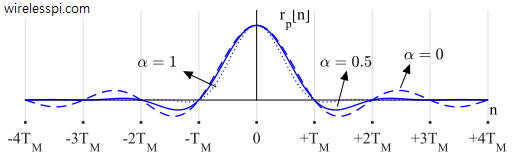
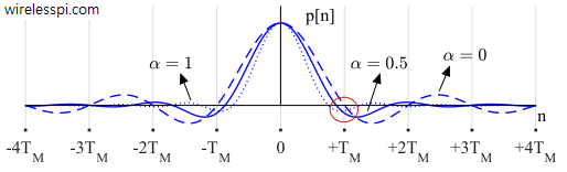
This is drawn in Figure below for different values of $\alpha$. Note the simultaneous zero crossings of all waveforms at integer multiples of $T_M$. Also, plugging $\alpha=0$ above produces the coefficients of a sinc signal, the same ideal Nyquist filter in Eq \eqref{eqCommSystemRectangleSinc}.

The above equation becomes indeterminate for $n=0$ and $n = \pm L/(2\alpha)$. It can be shown that (we skip the derivation and use a mathematical technique called L’H\^{o}pital’s rule)
\begin{align*}
r_p[0] &= 1 \\
r_p[\pm \frac{L}{2\alpha}] &= \frac{\alpha}{2} \sin \frac{\pi}{2\alpha}
\end{align*}

Resulting Pulse Shape

Until now in this section, everything we have discussed so far was about pulse auto-correlation that satisfies Nqyuist no-ISI criteria and is also called a Nyquist filter. However, how to derive the actual pulse shape is still not known. This is what we intend to find out next.

We start with a simple question: where should a Raised Cosine filter be placed in the system? There are only three possible choices.

[Receiver] The most straightforward way to incorporate it is to have it at the Rx. However, then a significant disadvantage is that there would be no mechanism to control the spectral sidelobes at the Tx. The spectral shaping required to minimize out-of-band energy cannot be avoided.

[Transmitter] If the spectrum is fully shaped at the Tx side, then any additional filtering at the Rx will not be “matched” to the incoming signal causing ISI. In the imaginary case of no filtering at all at the Rx, the noise and energy from adjacent channels will enter in the Rx in addition to unavoidable in-band noise. This significantly reduces the SNR as well as causing other issues such as increasing the interference sensitivity and dynamic range (adjacent channel energy can be quite higher than the desired band). So the Rx filter must be as compact as possible around the Tx spectrum so that maximal amounts of noise and adjacent channel interference can be eliminated.

[Both] The solution then is to split the Raised Cosine spectrum into two parts, one at the Tx to control the spectrum and the other at the Rx to reject noise and adjacent channels but still have zero ISI cumulative response. Remember that the pulse auto-correlation can be given by convolution formula as
\begin{equation*}
r_p(nT_S) = p(nT_S) * p(-nT_S)
\end{equation*}
The pulse shape $p(nT_S)$ can be placed at the Tx and its matched filter $p(-nT_S)$ at the Rx. Above, the response of two filters in cascade is the convolution of their impulse responses, which implies multiplication of their frequency responses.
\begin{equation*}
R_p (F) = P(F) \cdot P^*(F) = |P(F)|^2
\end{equation*}
From above equation, the frequency response of the actual pulse shape can be derived as
\begin{equation}\label{eqCommSystemPulseShape}
P(F) = \sqrt{R_p(F)}
\end{equation}
A significant advantage of this arrangement is that the matched filter simultaneously maximizes the Rx SNR.

In the case of Raised Cosine pulse auto-correlation, the underlying pulse shape is called Square-Root Raised Cosine (SR-RC) pulse or filter, where the square-root is in frequency domain. Referring to Eq \eqref{eqCommSystemRaisedCosineFreq}, taking the square-root does not affect $1$ and $0$ values. Using the identity $0.5(1+\cos 2\theta) = \cos ^2 \theta$ and taking the square-root on both sides adjusts the middle term as

\begin{equation}\label{eqCommSystemSR-RaisedCosineFreq}
P(F) = \left\{ \begin{array}{l}
1 \hspace{2in} 0 \le |F| \le 0.5(1-\alpha)R_M \\
\cos \left\{2\pi \frac{T_M}{4\alpha} \left( |F| – (1-\alpha)\frac{R_M}{2}\right)\right\} \\
\hspace{1.29in} 0.5(1-\alpha)R_M \le |F| \le 0.5(1+\alpha)R_M \\
0 \hspace{2.3in} |F| \ge 0.5(1+\alpha)R_M
\end{array} \right.
\end{equation}

For various values of excess bandwidth $\alpha$, this is shown in Figure below. For $\alpha = 0$, there is no difference between a Raised Cosine and a Square-Root Raised Cosine filter due to a rectangular spectrum. Also notice from Eq \eqref{eqCommSystemSR-RaisedCosineFreq} that the transition band of a Square-Root Raised Cosine pulse is a quarter cycle of a cosine as compared to a half-cosine of a Raised Cosine filter. It has implications which we shortly see.

Without mathematical derivation, the time domain waveform is given by
\begin{align}\label{eqCommSystemSR-RaisedCosineTime}
p[n] = \frac{1}{L}\cdot \frac{\sin \big[ \pi (1-\alpha) n/L\big] + 4\alpha n/L \cdot \cos \big[ \pi (1+\alpha) n/L \big]}{\pi n/L \big[ 1- (4\alpha n/L)^2\big]}
\end{align}

Figure below plots these time domain waveforms of Square-Root Raised Cosine for different values of $\alpha$. Observe again that plugging $\alpha=0$ produces a sinc signal, the same ideal Nyquist filter in Eq \eqref{eqCommSystemRectangleSinc}. Through the red ellipse in the figure, the zero crossings are seen at integer multiples of $T_M$ only for $\alpha=0$. For $\alpha =0.5$ and $\alpha=1$, Square-Root Raised Cosine does not satisfy Nyquist no-ISI criterion. This is not surprising because it has to fulfill that criterion only after matched filtering with another Square-Root Raised Cosine at the Rx to form the cumulative Raised Cosine shape.

In a software routine, the above equation can be used to find the coefficients of the Square-Root Raised Cosine pulse shape used for Tx filtering. Just like in Raised Cosine case, the denominator in this equation becomes zero for $n=0$ and $n = \pm L/(4\alpha)$. Pulse coefficients at these values can be given as (again, L’H\^{o}pital’s rule and skipping exact derivation}
\begin{align}
p[0] &= \frac{1}{L}\cdot \left(1 – \alpha + 4\frac{\alpha}{\pi} \right) \label{eqCommSystemSRRCPeakValue}\\
p[\pm \frac{L}{4\alpha}] &= \frac{1}{L}\cdot \frac{\alpha}{\sqrt{2}} \left\{ \left(1+\frac{2}{\pi} \right) \sin \frac{\pi}{4\alpha} + \left( 1-\frac{2}{\pi}\right) \cos \frac{\pi}{4\alpha} \right\}
\end{align}

Being a band-limited signal, the Square-Root Raised Cosine has is infinitely long in time that cannot be implemented in real systems. Therefore, it must be truncated to $G$ symbols to the left and $G$ symbols to the right. This is equivalent to $-LG \le n \le LG$ in samples, thus resulting in total filter length $N = 2LG+1$. This time span of $G$ symbols or $LG$ samples is called group delay (Group delay is a more general concept but this definition is good enough here).

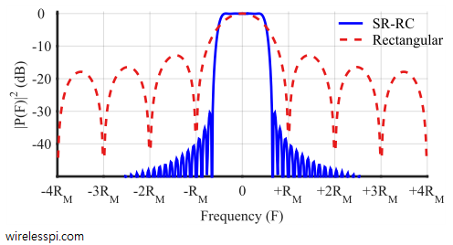
Figure below compares the spectra of a Square-Root Raised Cosine pulse with that of a rectangular pulse (rectangular in time, not frequency). The Square-Root Raised Cosine pulse is generated using $\alpha=0.25$, $L=8$ samples/symbol and $G = 4$ for a total filter length of $N = 2LG+1 = 65$ samples. The duration of rectangular pulse is obviously $8$ samples. A huge improvement in sidelobe suppression is fairly visible.

PAM Revisited

Let us now replace the Square-Root Raised Cosine filter above into our basic PAM system in place of a rectangular pulse. For a $2$-PAM modulation system with symbols $\pm A$, the process unfolds as follows. Keep comparing the signals thus generated with those from rectangular pulse shape.

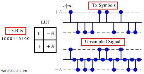
• A source generates Tx bits to be sent to a destination. These bits are input to a look-up table that maps bits to symbols according to a chosen modulation scheme. Next, the Tx symbols $a[m]$ are upsampled by $L=2$ samples/symbol. An example created of $10$ bits is illustrated in Figure below.

  

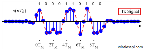
• The pulse shaping block with $L = 2$ samples/symbol, excess bandwidth $\alpha=0.5$ and group delay $G = 5$ symbols filters the waveform to output a smooth waveform $s(nT_S)$ which then is passed to the analog portion of the Tx. A DAC produces the continuous output $s(t)$ illustrated as dashed red line in Figure below. The bit information behind the waveform is also shown.

  

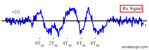
• In the best case scenario, i.e., a channel that only adds AWGN to the Tx signal, the Rx signal $r(t)$ is drawn as in Figure below.

  

• The Rx signal $r(t)$ is sampled by an ADC to produce $r(nT_S)$ and then input to a matched filter which is the same pulse shaping filter as at the Tx. The matched filter output $z(nT_S)$ at $L = 2$ samples/symbol is shown in Figure below. As long as the the combination of Tx and Rx filters (i.e., overall Raised Cosine filter) obeys Nyquist criterion, there is no ISI and one out of every $L$ samples at $n=mL = mT_M/T_S$ can be preserved to form a symbol estimate while the remaining $L-1$ samples are thrown away. If there was zero noise, these downsampled values directly map to the transmitted symbols without any error, from which the sequence of Rx bits can be found with the help of an LUT.

  

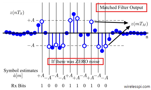
  To decide which one sample to keep out of every $L$ samples is the job of timing synchronization subsystem.

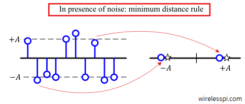
• When the noise is present which is always the case, the minimum distance rule is employed to produce symbol estimates $\hat a[m]$ according to its shortest distance from a constellation point, as illustrated in Figure below. Depending on numerous factors in system design, a proportion of bits will eventually end up in error, i.e., they will be different than Tx bits. The ratio of number of Rx bits in error to the total number of bits is called Bit Error Rate (BER).

  

Remember that in FIR filters, we said that every FIR filter causes the output signal to be delayed by a number of samples given by
\begin{equation}\label{eqCommSystemRCDelay}
\frac{\text{Length}\{h[n]\} – 1}{2} = \frac{LG}{2}
\end{equation}
and as a result, $LG/2$ samples of the output at the start — when the filter response is moving into the input sequence — can be discarded. Similarly, the last $LG/2$ samples — when the filter is moving out of the input sequence — should be discarded as well.

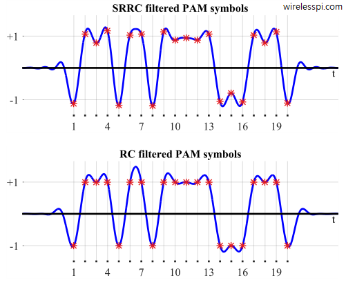
In summary, when the source information bits are filtered by a square-root Nyquist filter, the sharp edges visible for a rectangular pulse are smoothed out by a considerable margin, as shown in Figure below for 20 2-PAM symbols and excess bandwidth $\alpha = 0.5$. This smoothness in time domain actually limits the bandwidth. Also observe that in the absence of noise, the values at optimum sampling locations are not all the same and exhibit ISI in a square-root Nyquist case. This is because the zero crossings of a square-root Nyquist shape are not necessarily at integer multiples of symbol times. However, after complete Nyquist filtering and no noise, all values coincide with the same optimum symbol amplitudes shown as red asterisks in Figure below.

Coming back to our linear modulation framework where the pulse shape is scaled by a symbol and matched filter by the Rx, we have the following expression for the matched filter output.
\begin{equation*}
z(t) = \sum _{m} a[m] r_p(t-mT_M)
\end{equation*}
We can break this relation down to get two equivalent representations.
\begin{align*}
\sum _{i} a[i] r_p(t-iT_M) &= a[0]r_p(t) + a[1] r_p (t-T_M) + a[2] r_p(t – 2T_M) + \cdots \\
&= \Big( a[0] \delta(t) + a[1] \delta(t-T_M) + \\
&\hspace{1.5in}a[2] \delta (t-2T_M) + \cdots \Big) * r_p(nT_S)
\end{align*}
This is because convolution between any signal and a unit impulse results in the same signal. So far, we utilized the second expression involving the convolution in the above description. Now we have a look at the equivalent first relation for a deeper understanding. The unmodulated Nyquist pulse shapes (not square-root Nyquist) are drawn in Figure below. Notice the zero crossings of the $0^{th}$ pulse passing through
\begin{equation*}
T_M, 2T_M, 3T_M, \cdots
\end{equation*}
and so on, right at the peaks of the other pulse locations $t=mT_M$.

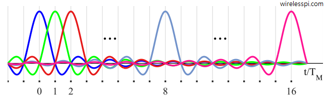
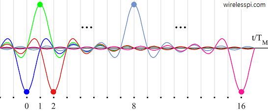
When a linear modulation scheme, such as BPSK, is utilized, the Nyquist pulse amplitudes are $a[m]=+1$ or $a[m]=-1$. The clock at the Rx then needs to sample at exactly the same instants $mT_M$, exhibiting zero ISI — maximum contribution comes from the desired pulse and zero contribution from all the rest. This is plotted in Figure below in the form of grid lines. In another article on role of timing synchronization, we will see how the presence of a timing offset causes the sampling in time domain at the wrong instants thus introducing ISI in the system.

Drawbacks of Square-Root Raised Cosine Pulse

As discussed above, Square-Root Raised Cosine pulse is much better than a rectangular pulse in shaping the spectrum but it has two major drawbacks.

[Insufficient Sidelobe Attenuation] There is a limit to the sidelobe suppression that a Square-Root Raised Cosine pulse can achieve. The sidelobe levels are reasonably higher than realistic spectral mask requirements imposed by regulatory authorities of attenuating out-of-band energy up to 60 to 80 dB. Looking back, recall that the transition band of a Raised Cosine pulse is half cycle of a cosine. Therefore, the transition band of a Square-Root Raised Cosine is a quarter cycle of a cosine, see Eq \eqref{eqCommSystemSR-RaisedCosineFreq} and spectrum of Square-Root Raised Cosine. Its abrupt termination at the stopband results in a discontinuity causing a relatively poor sidelobe response.

[Increase in ISI] Looking at spectral comparison of Square-Root Raised Cosine with a rectangular pulse, an important question arises at this stage: The spectrum of Square-Root Raised Cosine should be precisely $0$ beyond $0.5(1+\alpha)R_M$ Hz but why is it not? This is because as a consequence of truncation, the pulse is no more absolutely band-limited within $0.5(1+\alpha)R_M$ and assumes infinite support in frequency in the form of sidelobes. Remember that truncation means multiplication by a rectangular window. This multiplication between Square-Root Raised Cosine pulse and rectangular window in time domain is convolution between Square-Root Raised Cosine spectrum and a sinc signal in frequency domain (the sidelobes and in-band ripple are inherited from that oscillating sinc signal and are a function of excess bandwidth $\alpha$ and the pulse extension $G$ in symbols).
\begin{align*}
p_{\text{Truncated}}[n] &= p[n] \cdot w_{\text{Rect}}[n] \\
\quad P_{\text{Truncated}}(F) &= P(F) * sinc(F)
\end{align*}

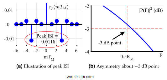
As a result of this truncation in time domain and subsequent convolution in frequency domain, the half amplitude values are moved away from the odd symmetry points of half symbol rate, or $F = \pm 0.5R_M$ as illustrated in Figure below. As a result, the spectral replicas now do not add up to exactly a constant value. In other words, Nyquist no-ISI criterion is only approximately satisfied by the truncated pulse shape, thus giving rise to increased ISI. The maximum magnitude of $r_p(mT_M)$ for $m \neq 0$ is called peak ISI, shown in Figure below to be equal to $-0.0115$ for excess bandwidth $\alpha = 0.5$ and group delay $G=3$.

The reader is encouraged to plot the spectra for different values of $\alpha$ and $G$ to appreciate their role in spectral shaping.

Square-Root Raised Cosine and Raised Cosine are good starting points for pulse shape design and capture the involved details fairly well. Moreover, they have closed-form mathematical expressions that are good for analytical purposes. Nevertheless, the quarter cycle cosine of the Square-Root Raised Cosine results in high in-band ripples and insufficient out-of-band attenuation levels. There are other pulse shape design procedures that produce a Nyquist filter with high sidelobe attenuation and preserve Nyquist no-ISI criteria as well.

A Frequency Domain Window Based Pulse

A spectral shape is a discrete-time signal and hence just a sequence of numbers. This sequence of numbers in time domain can be generated through iDFT of a carefully designed discrete-time frequency response. Recall that a Raised Cosine filter was generated in frequency domain through convolution of an ideal rectangular spectrum with a half-cosine taper. Here, we replace the half-cosine with an alternative taper that is an improved spectral window. The span of this spectral window is determined by the excess bandwidth $\alpha$ and the iDFT length.

The criteria for this spectral window design are

1. Narrow width of the mainlobe to effect a smoother transition band in resulting pulse spectrum. The width of the transition band remains unchanged
2. Small sidelobe levels that get inherited in the pulse spectrum

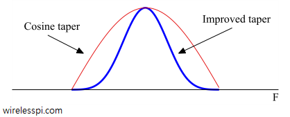
One such candidate is a Kaiser window in frequency domain (this technique is devised by Fred Harris in his paper “An Alternate Design Technique for Square-Root Nyquist Shaping Filters”) which has a minimum mainlobe spectral width for specified sidelobe levels. For a Kaiser window of a particular length, the sidelobe height is controlled by a parameter $\beta$. In Matlab, a Kaiser window of length $N$ with parameter $\beta$ can be generated through the command kaiser(N,beta). Figure below compares this taper with a cosine taper with the same transition bandwidth $\alpha = 0.25$ and highlights the difference of smoothness between the two.

In frequency domain, the convolution of this Kaiser window taper with an ideal rectangular spectrum generates the desired pulse shape. This frequency domain result is shown in Figure below for excess bandwidth $\alpha=0.25$ where it is compared with a Square-Root Raised Cosine pulse with the same excess bandwidth. This Figure depicts both the improved Nyquist filter and a Raised Cosine prior to square-root operation. Notice that a narrower mainlobe width of the improved taper has produced a smoother transition band in the improved Nyquist filter as compared to a Raised Cosine. This smoothness gets inherited by square-root Nyquist filter and it does not exhibit a similar kind of discontinuity as a Square-Root Raised Cosine, both of which are shown here. This discontinuity gives rise to high levels of time response even after many symbol intervals. When such an impulse response is truncated, it generates high sidelobes as well as in-band ripple in the spectrum of a Square-Root Raised Cosine. This is evident where an order of magnitude improvement in sidelobe suppression is visible. For example, an attenuation of $60$ dB is obtained through this procedure as compared to $40$ dB through Square-Root Raised Cosine.

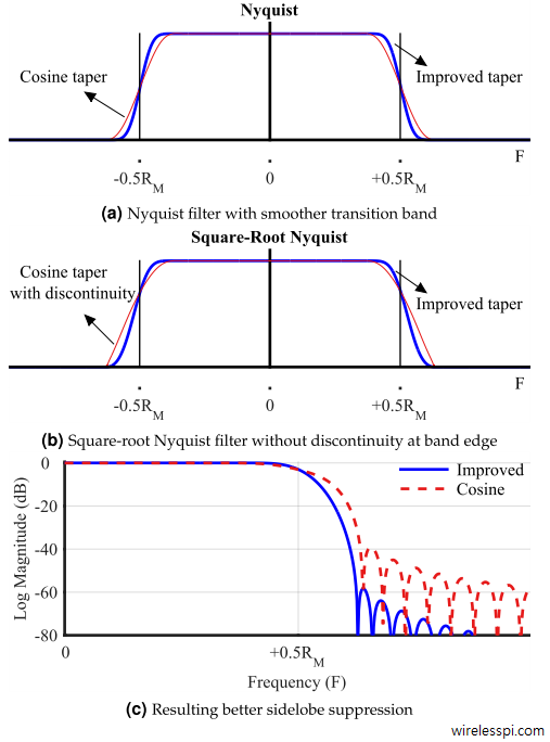
Not shown here is the fact that low levels of in-band ripple accompanies the low levels of sidelobes because they are always equal in a window based design (arising from convolution of the same spectral taper sliding through both stopband and passband). For reasons that are beyond the scope of this article, the low in-band ripple generates less ISI after matched filtering of the square-root Nyquist filter. Therefore, the additional advantage of sidelobe suppression comes with a benefit, not at a cost.

Finally, there are other pulse shape design procedures as well that employ iterative techniques to convert an initial lowpass filter to a square-root Nyquist filter with high sidelobe attenuation (from which a Nyquist filter can be obtained) while preserving Nyquist no-ISI criteria as well.